
Monte Carlo Method Explained
Before we talk about what a Monte Carlo Method is we need to understand some basics that will then allow us to use a Monte Carlo process to solve a simple example.
First let us look at a stock, this can be any stock traded anywhere on any exchange as fundamentally all stocks exhibit similar behaviour. The simple behaviour is that all stocks move up and down every day as they get traded. This implies that I can look at the move between yesterdays starting price and todays starting price and see if the stock went either up or down; this is effectively the 1 day vol. As you can imagine a stock may move a little day to day but some days they can move significantly more than other days. This is why rather than 1 day vol we usually look at a stock across many days or even a whole year in order to work out the vol or volatility of the stock. That is the theory but in practice vol is not static on a stock and the vol can go up and down as the stock has bigger price swings from day to day or smaller price swings day to day, hence why in the real world we are likely to use a vol surface for the computation but to keep it simple we will suspend this and assume vol to be annualised and fixed for the year. You should also bear in mind that this can be referred to as Sigma as that is the greek sign used in Finance.
Secondly let us look at the return on investment. Why would you buy an investment unless it was your belief that the investment would go up in value? This is the annualised return sometimes called mu. So if a stock has a rate of return of 5% then provided there are no major market moves to the down side or large events you would expect to receive 5% on your investment at the ned of 1 year assuming you simply bought the stock ( This means you are long the Stock). This is the annualised rate of return or mu.
Now we have volatility ( vol ) and mu ( annualised rate of return ) we can start talking about how we can use these in a Monte Carlo example. If we consider the price movement of 1 stock let us call this S. The starting price at day one is 100 and we will use a vol which we sometimes cal sigma of 20% or .2 and we expect an annualised return or mu of 5% or .05. Then we do a simple random walk ( By Random I mean the Normal Random Distribution ) which looks at the change in price across the next 250 days ( There are roughly 250 business days in a year excluding weekends ) then we would get a picture similar to the ones below:
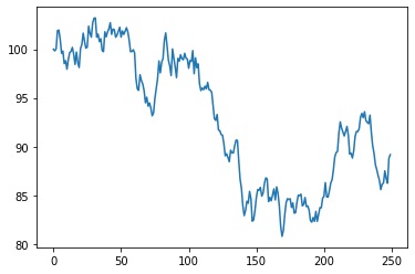

You may ask why we have 2 different paths the price starts at 100 but the paths are totally different. This is the key to the Random or Normal Distribution, every time we do a calculation, or simulate a stock movement over time, you get a different answer or a different path. Now if I did this 10,000 times and graphed each of the paths or Random Walks together it would look like this:
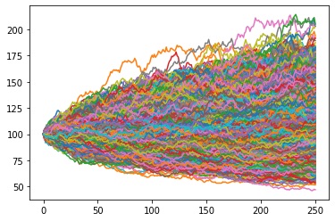
Notice that we started all the paths at S=100 but the randomness of Vol or sigma caused us to have many different outcomes. I am sure the statistician in you is now thinking "hey I can perhaps take the results split them into bins and create a normal distribution" and you would be correct. I am not going to go into detail about statistics but essentially you take the highest result and the lowest result and create 100 equal number ranges between them or 100 bins and then do a count of how many fell into that number space. For example if I had numbers rating from 0 to 100 split into 10 bins I would have 10 bins of 10 ie 10*10=100 now I count how many simulations or paths are in bin range 1-10 and bin 1 would take that count, now do the same for all other bins.
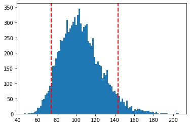
Once I split the above into 100 bins I get this approximate distribution. It is not smooth as I would need more than 100K results and a lot more bins to make it smoother but you get the idea.
I can then graph these bins each vertical bar in the distribution graph represents the count of the simulations in that bin.
Once I have the distribution I can then take the mean and the 5th Quantile or Percentile and the 95th Quantile.
Mean is 105.23087453735496
5% quantile = 74.39391341531278
95% quantile = 143.31363983253607
This in essence is the idea of using a Monte Carlo for problem solving. It is the fact that we have to do so many simulations, here Random Walks, that allows this process to be computed in a Multi Processor or Multi Threaded way.
Just on 10K simulations we are starting to converge on 5% ie 105.23 as the mean which we would expect as the Stock has a 5% annualised return.
A talk on Monte Carlo would not be complete if I did not also provide you with some Caveats that you must take into account when solving a problem this way.
What is Random
This is a large and complex topic so I will only provide you some food for thought. If you are using a computer to calculate the random variable is it truly random. A computer uses an algorithm so if you work out what that is you could effectively rig the result. If you were to look on wikipedia you will see plenty of mathematical notation for what makes a good random number generator and how to generate random numbers. Here i use numpty random for python or a Mersenne Twister in Java which provides me with random enough results but you should think about this if you are writing a Monte Carlo for real world use.
What is Convergence
When we did the calculations above why did I use 10K simulations. I could have used 100K or 1 Million. The question comes down to when does the averaging function have enough data so that the deviation of the mean does not change significantly the more simulations you provide. Indeed having too many simulations wastes compute time, too few simulations will give you an answer that may not be the true average. So how do you find convergence of mean ? Unless you know the answer up front as we do here, you run as many simulations as you need to get there. In the real world you can do a continuous mean calculation and check if the mean is only changing by a specified error margin say 4 decimals then you can assume you have convergence. This may mean you don't know how many simulations you will need up front.
Is the Normal Distribution suitable given it does not have a Fat Tail
The Normal distribution has been used since the beginning of Black Scholes in Finance as far back as the 1970's. It was always assumed that prices behaved stochastically and conformed to the Normal distribution. Recently however with far more data we are starting to question this fundamental assumption, because if you look at a distribution of Stocks since the early 1900's it seems that it is not quite as Normal as we had all assumed. There is a lot of literature and further reading available on Fat Tails if you are interested but it would be beyond the scope of this article to explain the details. The important thing is that this is effectively an assumption we make in Finance that may come back to haunt us someday.
What problems can be solved with Monte Carlo
When we try to price things like non Path dependant derivatives or simple vanilla derivatives then there are closed form partial differential equations or PDE's that allow us to arrive at an answer fairly quickly such as the Black Scholes PDE. ( Follow this link where I explain it in a bit more detail) However if you are an Exotic derivative you will effectively be path dependant ie: a Barrier option that knocks out or knocks in at a certain level is discontinuous so you can not use Black Scholes or closed form PDE's. Any pricing requirement or Risk calculation that requires you to run many simulations would be a candidate for Monte Carlo. There is a Warning however, and that is Monte Carlo is a heavy weight process in that it requires many simulations and a lot of compute time. Certain calculations especially exotic derivatives may be better done using a FDM or Finite Difference Model and this would be faster than a Monte Carlo. So never assume a Monte Carlo is always the best solution it is one of many algorithms that we can use.
Is there a Python Code example demonstrating the Monte Carlo process
There is some straightforward Python Code that I used to create all the Graphs above, the code is not threaded and it takes a while to run. You can run it faster by only running 1000 simulations rather than 10K.
For a threaded python version see This link
Is there a Multi Threaded Java example of Monte Carlo
The Java code class here will use a MersenneTwister random number generator and creates a Random Walk. This code is from my Private Quant library that I wrote to get a grip on how things actually work in Finance as its one of my passions. The code uses a Java CompletionService and a CachedThreadPool.
HOME

Naive Bayes classification AI algorithm
K-Means Clustering AI algorithm
Equity Derivatives tutorial
Fixed Income tutorial
Java
python
Scala
Investment Banking tutorials
First let us look at a stock, this can be any stock traded anywhere on any exchange as fundamentally all stocks exhibit similar behaviour. The simple behaviour is that all stocks move up and down every day as they get traded. This implies that I can look at the move between yesterdays starting price and todays starting price and see if the stock went either up or down; this is effectively the 1 day vol. As you can imagine a stock may move a little day to day but some days they can move significantly more than other days. This is why rather than 1 day vol we usually look at a stock across many days or even a whole year in order to work out the vol or volatility of the stock. That is the theory but in practice vol is not static on a stock and the vol can go up and down as the stock has bigger price swings from day to day or smaller price swings day to day, hence why in the real world we are likely to use a vol surface for the computation but to keep it simple we will suspend this and assume vol to be annualised and fixed for the year. You should also bear in mind that this can be referred to as Sigma as that is the greek sign used in Finance.
Secondly let us look at the return on investment. Why would you buy an investment unless it was your belief that the investment would go up in value? This is the annualised return sometimes called mu. So if a stock has a rate of return of 5% then provided there are no major market moves to the down side or large events you would expect to receive 5% on your investment at the ned of 1 year assuming you simply bought the stock ( This means you are long the Stock). This is the annualised rate of return or mu.
Now we have volatility ( vol ) and mu ( annualised rate of return ) we can start talking about how we can use these in a Monte Carlo example. If we consider the price movement of 1 stock let us call this S. The starting price at day one is 100 and we will use a vol which we sometimes cal sigma of 20% or .2 and we expect an annualised return or mu of 5% or .05. Then we do a simple random walk ( By Random I mean the Normal Random Distribution ) which looks at the change in price across the next 250 days ( There are roughly 250 business days in a year excluding weekends ) then we would get a picture similar to the ones below:
You may ask why we have 2 different paths the price starts at 100 but the paths are totally different. This is the key to the Random or Normal Distribution, every time we do a calculation, or simulate a stock movement over time, you get a different answer or a different path. Now if I did this 10,000 times and graphed each of the paths or Random Walks together it would look like this:
Notice that we started all the paths at S=100 but the randomness of Vol or sigma caused us to have many different outcomes. I am sure the statistician in you is now thinking "hey I can perhaps take the results split them into bins and create a normal distribution" and you would be correct. I am not going to go into detail about statistics but essentially you take the highest result and the lowest result and create 100 equal number ranges between them or 100 bins and then do a count of how many fell into that number space. For example if I had numbers rating from 0 to 100 split into 10 bins I would have 10 bins of 10 ie 10*10=100 now I count how many simulations or paths are in bin range 1-10 and bin 1 would take that count, now do the same for all other bins.
Once I split the above into 100 bins I get this approximate distribution. It is not smooth as I would need more than 100K results and a lot more bins to make it smoother but you get the idea.
I can then graph these bins each vertical bar in the distribution graph represents the count of the simulations in that bin.
Once I have the distribution I can then take the mean and the 5th Quantile or Percentile and the 95th Quantile.
Mean is 105.23087453735496
5% quantile = 74.39391341531278
95% quantile = 143.31363983253607
This in essence is the idea of using a Monte Carlo for problem solving. It is the fact that we have to do so many simulations, here Random Walks, that allows this process to be computed in a Multi Processor or Multi Threaded way.
Just on 10K simulations we are starting to converge on 5% ie 105.23 as the mean which we would expect as the Stock has a 5% annualised return.
A talk on Monte Carlo would not be complete if I did not also provide you with some Caveats that you must take into account when solving a problem this way.
What is Random
This is a large and complex topic so I will only provide you some food for thought. If you are using a computer to calculate the random variable is it truly random. A computer uses an algorithm so if you work out what that is you could effectively rig the result. If you were to look on wikipedia you will see plenty of mathematical notation for what makes a good random number generator and how to generate random numbers. Here i use numpty random for python or a Mersenne Twister in Java which provides me with random enough results but you should think about this if you are writing a Monte Carlo for real world use.
What is Convergence
When we did the calculations above why did I use 10K simulations. I could have used 100K or 1 Million. The question comes down to when does the averaging function have enough data so that the deviation of the mean does not change significantly the more simulations you provide. Indeed having too many simulations wastes compute time, too few simulations will give you an answer that may not be the true average. So how do you find convergence of mean ? Unless you know the answer up front as we do here, you run as many simulations as you need to get there. In the real world you can do a continuous mean calculation and check if the mean is only changing by a specified error margin say 4 decimals then you can assume you have convergence. This may mean you don't know how many simulations you will need up front.
Is the Normal Distribution suitable given it does not have a Fat Tail
The Normal distribution has been used since the beginning of Black Scholes in Finance as far back as the 1970's. It was always assumed that prices behaved stochastically and conformed to the Normal distribution. Recently however with far more data we are starting to question this fundamental assumption, because if you look at a distribution of Stocks since the early 1900's it seems that it is not quite as Normal as we had all assumed. There is a lot of literature and further reading available on Fat Tails if you are interested but it would be beyond the scope of this article to explain the details. The important thing is that this is effectively an assumption we make in Finance that may come back to haunt us someday.
What problems can be solved with Monte Carlo
When we try to price things like non Path dependant derivatives or simple vanilla derivatives then there are closed form partial differential equations or PDE's that allow us to arrive at an answer fairly quickly such as the Black Scholes PDE. ( Follow this link where I explain it in a bit more detail) However if you are an Exotic derivative you will effectively be path dependant ie: a Barrier option that knocks out or knocks in at a certain level is discontinuous so you can not use Black Scholes or closed form PDE's. Any pricing requirement or Risk calculation that requires you to run many simulations would be a candidate for Monte Carlo. There is a Warning however, and that is Monte Carlo is a heavy weight process in that it requires many simulations and a lot of compute time. Certain calculations especially exotic derivatives may be better done using a FDM or Finite Difference Model and this would be faster than a Monte Carlo. So never assume a Monte Carlo is always the best solution it is one of many algorithms that we can use.
Is there a Python Code example demonstrating the Monte Carlo process
There is some straightforward Python Code that I used to create all the Graphs above, the code is not threaded and it takes a while to run. You can run it faster by only running 1000 simulations rather than 10K.
For a threaded python version see This link
import numpy as np
import math
import matplotlib.pyplot as plt
from scipy.stats import norm

#Define Variables
S = 100
T = 250 #Number of trading days
mu = .05 #Return or Compound Annual Growth rate
vol = .2 #Volatility or Sigma
result = []

#choose number of runs to simulate - I have chosen 1000
for i in range(10000):
    #create list of daily returns using random normal distribution
    daily_returns=np.random.normal((mu/T),vol/math.sqrt(T),T)+1
    #Parameters: for np.random.normal
    #Mean (“centre”) of the distribution.
    #Standard deviation (spread or “width”) of the distribution.
    #size : int or tuple of ints, optional

    #set starting price and create price series generated by above random daily returns
    price_list = [S]

    for x in daily_returns:
        price_list.append(price_list[-1]*x)

    #plot data from each individual run which we will plot at the end
    plt.plot(price_list)
    #catch last value in the simulation
    result.append(price_list[-1])
#show the plot of multiple price series created above
plt.show()


#Distribution
plt.hist(result,bins=100)
plt.show()
#npRes=np.array(result)
print("Mean is ",np.mean(result))

print("5% quantile =",np.percentile(result,5))
print("95% quantile =",np.percentile(result,95))

plt.hist(result,bins=100)
plt.axvline(np.percentile(result,5), color='r', linestyle='dashed', linewidth=2)
plt.axvline(np.percentile(result,95), color='r', linestyle='dashed', linewidth=2)
plt.show()
Is there a Multi Threaded Java example of Monte Carlo
The Java code class here will use a MersenneTwister random number generator and creates a Random Walk. This code is from my Private Quant library that I wrote to get a grip on how things actually work in Finance as its one of my passions. The code uses a Java CompletionService and a CachedThreadPool.
/**
*
* @author arifjaffer
*/
public class MySpecialMCRandomWalk implements MCRandomWalkerInterface{
private volatile double res=0;
double asset=100;
double IR=.05;
double vol=.2;
double dt=1.0/100.0;
double mu=.1;
Random generator = new Random();
//not ideal but we want each twister to have a different seed as many threads of this class can start simultaneously
// the twister just seeds you based on current time in milliseconds which could be the same for many threads
MersenneTwister mt = new MersenneTwister(generator.nextInt());
public void Walk(){
double dX=0;
double dS;
for (int t=1; t<=100; t++) {
//use Defined Random Generator or The Java Gaussian
//dX=Normal.normal(1.0, 0.0)*Math.sqrt(dt);
dX=mt.nextGaussian()*Math.sqrt(dt);
//dX=generator.nextGaussian()*Math.sqrt(dt);
dS=asset*((IR*dt)+(vol*dX));
asset+=dS;
//if you want to use a different SDE modify teh dS
}
res=asset;
}
public synchronized double getRes(){
return res;
}
}
// Here is the Interface
/**
*
* @author arifjaffer
*/
public interface MCRandomWalkerInterface {
public void Walk();
public double getRes();
}
//Here is the Controller that runs it all
/**
*
* @author arifjaffer
*/
public class MCController {
private double Avg=0.0;
private final ExecutorService executor = Executors.newCachedThreadPool();
public long lcompleted=0;
private ArrayList resList = new ArrayList();
public void MCme(long lSims){
CompletionService completionService = new ExecutorCompletionService( executor);
for(int i=0; i<lSims; i++){
System.out.println("call "+i+" ");
completionService.submit(new Callable() {
public MySpecialMCRandomWalk call() throws Exception {
final MySpecialMCRandomWalk rw = new MySpecialMCRandomWalk();
rw.Walk();
return rw;
}
});
}
try{
for( int t=0; t<lSims; t++){
Future f = completionService.take();
MySpecialMCRandomWalk rw = (MySpecialMCRandomWalk) f.get();
lcompleted = t;
System.out.println(t +": "+ rw.getRes()+"\n");
resList.add(rw.getRes());
}
//create avg
double sum=0;
for(int i=0; i<resList.size(); i++) {
sum+=resList.get(i);
}
System.out.println("Average is: " + sum/resList.size());
Avg=sum/resList.size();
}catch(InterruptedException e){
Thread.currentThread().interrupt();
}catch(ExecutionException e){
System.out.println(e.getMessage());
//throw e;
}finally{
;
}
}
public synchronized double getAvg(){
return Avg;
}
}
HOME
People who enjoyed this article also enjoyed the following:
Naive Bayes classification AI algorithm
K-Means Clustering AI algorithm
Equity Derivatives tutorial
Fixed Income tutorial
And the following Trails:
C++Java
python
Scala
Investment Banking tutorials