
Equity Derivatives
Filed in: Derivatives | Delta | Gamma | Theta | Vega | Rho | Put Call Parity | Banking | Finance | Vol Smile
Before diving into how to value an Option we must first realise that in this discussion we are only looking at non path dependant options. These are options that are European and that will expire on a set date. We are also looking at vanilla options with no embedded decisions or other attributes that would change their payouts and make them exotic.
Derivatives is a name we usually give to something where we derive the value from an underlying. Here we will look at Stock being the underlying and the Option will be the Derivative on that underlying. Since we are talking about stocks you need to realise that a stock price moves from day to day and the daily movements be they up or down can effectively be seen as a Random walk through time with drift. The element of drift is down to the fact that Stock prices from day to day tend to move up and down but in the longer term the hope is that all stock prices will drift upwards. The daily movements can be seen as the variance of the stock and in fact the whole of Black Scholes is predicated against the fact that these movements can be statistically assessed and will fit into a normal statistical distribution. The normal distribution means that you go up as well as down and if you take all these movements and take the standard deviation you can effectively start to plot a bell curve.
A word of caution though needs to be sounded at this point. Even though Black Scholes uses the Normal distribution we all know that the distributions in the real market as opposed to the theoretic maths tend to have fat tails. We also know that Volatility the size of the ups and downs are not static over time as they must be for the theoretic Black Scholes but volatility tends to vary over time.
Now that we can plot the stock movements into a Normal distribution we find that the stock moves are akin to Geometric Brownian motion.
With this in mind we can now look at the formula for Black Scholes.
The simplest way to understand this partial differential equation is to realise we are talking about movements in three dimensions. This version of the equation is = 0 but we could solve it for the value of the option and then we are talking about the value of the option depending on time t, Stock S, r is the risk free rate, and sigma is the vol.
We can then say that the value of an option is dependant on theta + Gamma + risk free rate Stock(rS) * Delta - risk free rate * value of the option.
This is where we get the greeks in derivatives from, so lets talk a bit about the greeks and what they mean.
Theta - the time value of an option or the time decay of the value of the option. The closer to expiry the bigger the time decay so the less valuable the option is.
Delta - the rate of change of the value of the option based on movements in the stock. This can be seen as the hedging amount. how much do you need to hedge or how much stock do you need to buy to keep your position flat.
Gamma - the second derivative the first being Delta. This is how big a delta move is going to be and also implies how often you will need to hedge to keep flat. The higher the Gamma the more you need to hedge.
Vega - sensitivity to volatility or the change in the option Value with respect to volatility of the underlying asset.
Rho - sensitivity of the price of the option with respect to basis points move in the risk free rate.
There are a few others but these are the main greeks.
Put Call Parity
No discussion would be complete without talking about Put Call Parity. So far I have not said if I am talking about a put option or a call option. In theory they are the same except for a put option you are looking at negative numbers relative to the strike. We have also talked about the theoretic version of Black Scholes and most banks will have a discretised version that calculates the value given a specific strike.
When we talk options we usually talk about then in terms of a hedging strategy where we either hold the stock or we do not. The put call parity is the theory that says:
Long call (C) and a short put (-P)= Underlying(1) * risk free rate
or a shorthand way of remembering is this
C - P = 1
Given the put call Parity you can now create different hedged and unhedged strategies.
Assumptions in Black Scholes
I need to make clear that Black Scholes does have some downsides and almost no bank will use it in its theoretic form. However they will extend it to add extra features and give it real world assumptions. These details are beyond the scope of this discussion and usually proprietary.
The equation assumes no dividends are returned in the time period for the stock. Though you could update the equation to include it.
Risk free rate is constant over the time period. Most real world equations will expect a rate curve to overcome this drawback.
The time period is fixed so you can only use Vanilla Europeans in theoretic valuation. However you can value American Vanilla options using Finite Difference models and others which have grown out of the Black Scholes theory.
Volatility is fixed for the time period. Most real world applications will require you to provide a volatility surface to overcome this. When using theoretic Black Scholes you need to give a specific Volatility number that you have derived through some approach such as GARCH or Weighted Vol.
Using Black Scholes to find the Volatility Smile.
The volatility smile is the observed volatility in the market for different options both greater than the strike and less than the strike. Say you had a strike (K) at 100 you would look 3% below and above that strike for options with the same Expiry and 5% below and above that strike for options with the same expiry. You now have 5 options. These are K-5%, K-3%, K, K+3%, K+5% and you would solve Black Scholes for sigma so you now have an equation that says Sigma =. This means you already know the market observed values of the option as you have the strikes above. You plug in these values and solve the equation 5 times and plot the Implied Volatility against the Strikes. This implied or market observed or market derived volatility is what gives you the smile. Note in Equites it is more of a skew and in FX it is more of a smile but it is the same theory.
In order to show this Graphically Consider the following European Call option Stock Price = 100 Strike = 100 meaning it is at the money. Volatility 20% expires in .1 of a year or about 36 Days with Risk free rate of 5% no dividend Yield.
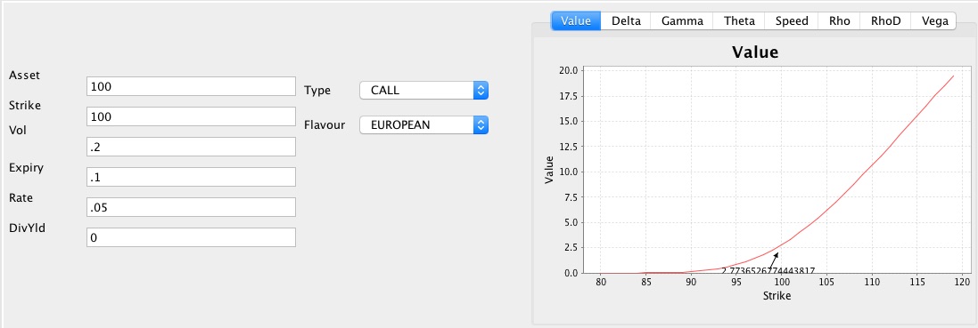
Then you get a value of 2.77 as shown in the graph. The delta then looks like this
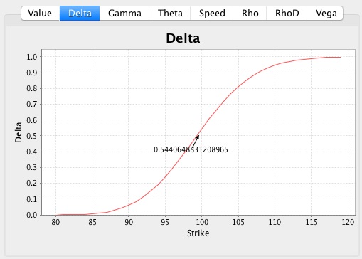
The graphics are from my own Quant Library.
People who enjoyed this article also enjoyed the following:
Naive Bayes classification AI algorithm
K-Means Clustering AI algorithm
Equity Derivatives tutorial
Fixed Income tutorial
Monte Carlo Explained
And the following Trails:
C++Java
python
Scala
Investment Banking tutorials
HOME
